
Towards Quantum Computing (III): Through the Quantum Gate
Let's discover how we process qubits. In this post we'll learn about the building blocks of quantum algorithms.

If you missed the previous chapter of the series, don’t worry, I got you covered:
Towards Quantum Computing (II): The Secure Quantum Channel

Missed the previous chapter of the series? I got you covered: Hello, Hypers! Let’s continue our series on Quantum Computing. In the previous chapter, we learned about the two main properties of particles that can be useful for computation: superposition
Hello, Hypers!
Ready for another chapter of our quantum series? I would love to start doing some quantum algorithms together but you know here in Under the Hype we try to be rigorous. Thus, we’ll first learn the building blocks of quantum algorithms.
Note: I included many handwritten notes in this post so it is a bit heavier than the previous ones. Maybe your e-mail client has truncated it but don’t worry, you’ll still be able to read it entirely. That’s great because I’m keeping the best part for the end!
You probably know that bits are the tiniest unit of information in classical computers. A bit can be either zero or one. Classical algorithms operate on bits. There is a set of fundamental operators like NOT, AND, OR, NAND, etc. You have probably heard about them.
These operators are also called gates; we can simulate them with electronic circuits. The computer where I’m writing this exciting chapter of our series on Quantum Computing is, more or less, a collection of electronic circuits with millions of these gates.
But if you have been following this series, then you also know that qubits are different from bits. In general, they are in a superposition of the states zero and one, and they can be entangled together (although we haven’t talked too much about entanglement yet if you keep reading this post I have a little surprise at the end).
It is reasonable to think that we would require special gates to create quantum algorithms, and that is exactly the case. In this post, we’ll learn about quantum gates. They are the building blocks of quantum algorithms. But first, we need to agree on some notation.
Notation to work with qubits
We need a special notation to work with qubits. How do we write a superposition between zero and one? Are all the superpositions the same? Let’s talk about the notation we are going to use in this post.
We can imagine a superposition as a probability distribution. At each instant, a qubit has a probability to be zero and a probability to be one. Measuring the state of a qubit makes the superposition collapse into either zero or one, but it could be more likely to be zero than one or vice-versa. It all depends on the probabilities of the superposition.
Then, we are going to write the superposition of a qubit using what is called the Bra-Ket notation proposed by Dirac. In general, the state of a qubit will be denoted by:
Where a and b are numbers. There are two funny guys in this formula:
These are the zero and one states respectively. The numbers a and b can be seen as the probabilities to be zero and one respectively.
Note: The coeficients (the numbers
aandb) are not exactly probabilities. In general, they are complex numbers. We’ll dedicate an entire post to explain exactly what a qubit is from a mathematical perspective. But for now, let’s say they are probabilities.
As the states zero and one are fixed for a qubit, the superposition is entirely determined by the 2D vector (a b). There is a huge difference between this vector representation (the qubit representation) and the zero-one representation of a bit. That’s why the classic NOT, AND, and OR gates won’t work in Quantum Computing.
What do the quantum gates look like?
A matrix is all you need
Transformations on qubits are represented by matrices. Specifically, 2x2 orthonormal matrices. If you want to know more about matrices and what an orthonormal matrix is, check The Palindrome, a publication by Tivadar Danka that has several posts exploring matrices in a fascinating way.
For now, it is enough to know that a matrix can have an associated inverse matrix with the following property:
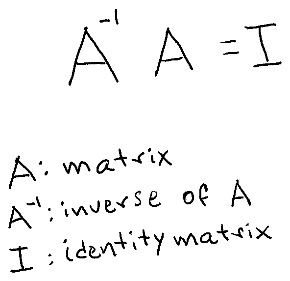
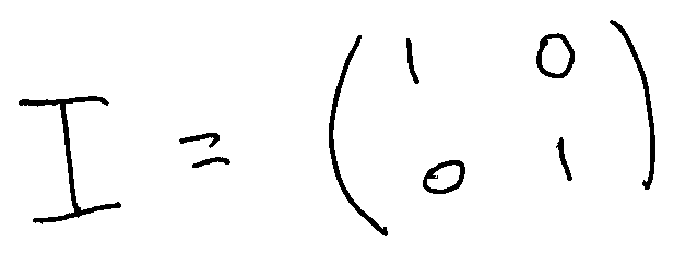
The identity matrix is a special one. If we multiply any matrix A with the identity matrix, we’ll get the matrix A again. In Quantum Computing, qubits are in a superposition of two states, so the matrices we are going to work with have two rows and two columns (2x2 matrices). The identity 2x2 matrix is:
All matrices have associated yet another matrix called the transpose. To calculate the transpose of a matrix we just need to write the columns like the rows and vice-versa. For example:
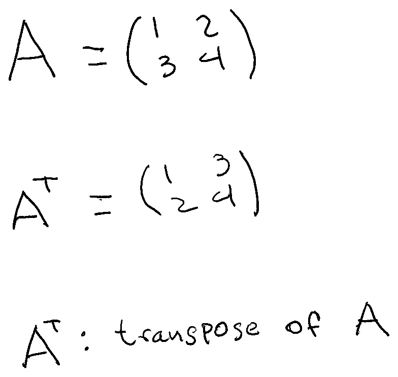
And now a last piece of knowledge about matrices: if a matrix is orthonormal, then its inverse and its transpose are the same matrix.
This makes it very easy to calculate the inverse matrix. In Quantum Computing, the gates to operate on qubits are orthonormal matrices. We multiply these matrices to apply the transformations. As the matrices are orthonormal, they will always have an inverse matrix and it is easy to calculate that inverse matrix. This means that all quantum operations are reversible.
To understand this, let’s recall what the classic AND operation looks like. The AND gate is applied to two bits. When both bits are one, the AND operation returns a one, otherwise, it returns a zero. Now imagine you know the result of an AND operation is zero, what were the input bits?
There is no way to know if both bits were zero or if one of them was one. The AND operation is not reversible. In general, there is no way to recover the input from the output. That won’t happen with quantum gates. We can always multiply by the inverse of an operation and recover the initial qubits.
All of this is fine, but it seems we got too theoretical, and now we don’t know why are we talking of matrices in the first place. Ok, they are the gates of the Quantum World, but what are the transformations we can apply with them? Let’s discover it now!
Examples of quantum gates
Let’s begin with the simplest one: the Quantum NOT. Classical NOT convert a one into a zero and vice-versa. As qubits are in a superposition of one and zero, the Quantum NOT will swap the probabilities of both states:
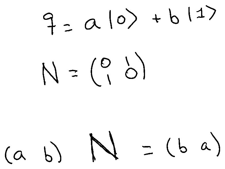
If we multiply the vector of the coefficients of a qubit by the matrix N we’ll get the vector with the coefficients swapped. The matrix N is the Quantum NOT. As it is its same transpose, the inverse of N is N itself. So, applying N two times we get the same input qubit.
Another important transformation is the Hadamard Gate. This gate converts a zero or one qubit into a qubit in a superposition of the two states. For example, we can pass a qubit that is not in superposition and is equal to zero and obtain a qubit in a superposition of 50% zero and 50% one.
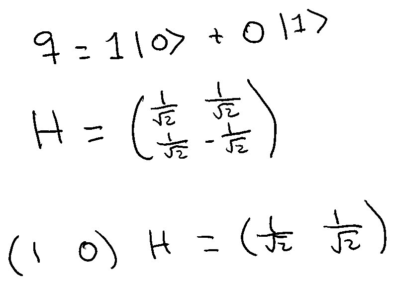
Matrix H creates the superposition. In this example, we used a qubit in the zero state but the same happens when the input is a qubit in the one state. The Hadamard Gate is also its own inverse, so by applying it two times, we get the initial qubit.
The last single-qubit gate we are going to learn about is the Z-Gate. This is an easy one, it flips the sign of the coefficient of the one state. Remember that the coefficients are not exactly probabilities so having negative coefficients is normal. We’ll learn more about these coefficients in a future post.
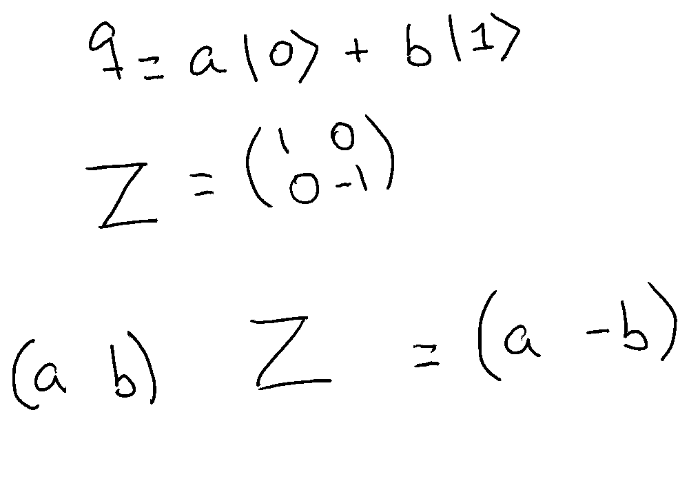
Again, matrix Z is its own inverse.
Now let’s see one last example. Until now, we have been talking about single-qubit gates. Those were gates with a single qubit input. But it is possible to have a gate that acts on multiple qubits. For example the CNOT Gate. CNOT comes from Controlled NOT. This gate receives two qubits, one of them is called the control qubit, and the other one is the target qubit. The control qubit is not modified at all, and the target qubit is modified following these two rules:
If the control qubit is zero, then the target qubit is not modified.
If the control qubit is one, then the target qubit is flipped from zero to one or from one to zero.
This way of defining the CNOT Gate seems too classical in the sense that we are talking about zero and one state. However, the CNOT Gate is applied to every state of the input qubits. To understand this, we first need to talk about the different states in a multi-qubit system.
Now we have two qubits that are in a superposition of two possible states. So, the entire system is in a superposition of four possible states.
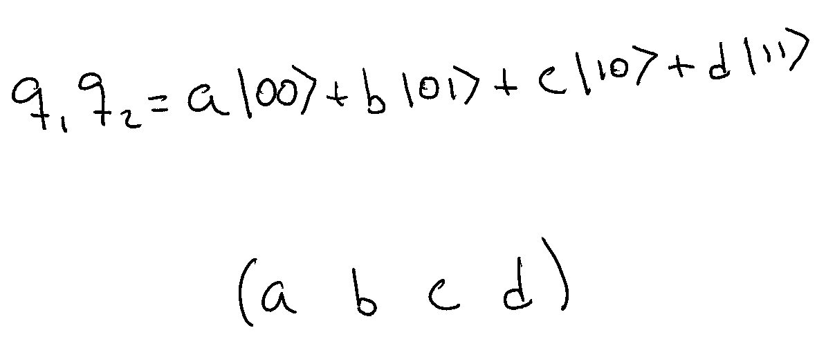
Now the representation of the whole system is a vector with four coefficients and the CNOT Gate is represented by a 4x4 matrix
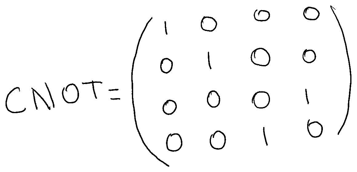
If, for example, the control qubit is in a 50-50 superposition of zero and one, and the target qubit is collapsed to zero, then we have the following result:
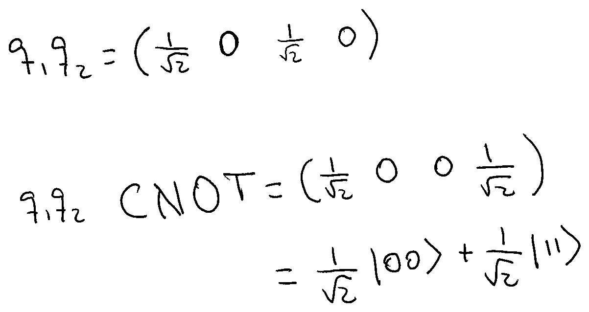
The resulting system has a 50% chance of being zero-zero and a 50% of being one-one. We don’t know what values we’ll obtain for both qubits if we measure them but we know both qubits will have the same value. They are entangled!
With the CNOT Gate, we can create entangled systems of qubits. If after applying this CNOT Gate as we did before, Alice takes one of them to Neptune, measures it there, and gets a one, then the other qubit will immediately turn into a one too. This is the mindblowing result of Quantum Mechanics.
The CNOT gate is again its own inverse so we can obtain the initial state of the system by applying it two times.
Conclusion
Quantum Gates are the transformations we apply to qubits. They can be represented by orthonormal matrices. This is important because it means all the quantum operations are reversible and we can always obtain the initial input from the output.
We learned about single-qubit gates like the Quantum NOT, the Hadamard Gate, and the Z-Gate. Also, we learned how to work with multiple-qubit systems and the CNOT Gate that allows us to entangle two qubits.
This was quite a ride to introduce quantum gates. As we said before, these are the building blocks of quantum algorithms. If you are enjoying this series let me know by commenting and hitting the heart button of this post. I’m always open to writing about any topic related to Computer Science so don’t be shy and tell me what you’d like to read about. Don’t forget to share Under the Hype with your friends.
That’s all for today, see you next Tuesday!