

Towards Quantum Computing (V): Season Finale
Towards Quantum Computing (V): Season Finale
Let's implement our first quantum algorithm. Not just in paper, we are going to write some code!

Hello, Hypers!
This is the last post of the first season of the Towards Quantum Computing series. It has been quite a journey and there are still a lot of things to discover. That’s why we’ll come back to talk about qubits and superposition after a pause. So far, we have learned:
The principles of quantum mechanics that make Quantum Computing interesting: superposition and entanglement.
An application of Quantum Computing in Cryptography.
Quantum Gates.
Pros and Cons of Quantum Computing.
Did you miss the previous chapter? I've got you covered:

In this chapter, we are going to implement our first quantum algorithm. So, let’s get started!
Problem statement
As we saw in the previous chapter, quantum computers are good just for some kinds of problems. The following problem is an example of a case in which quantum computers can be faster than classical computers.
Let f(x) be an unknown function that operates on a single bit/qubit and outputs either zero or one. There can only be four different functions that satisfy this requirement. Those functions are:
f(0) = 0 and f(1) = 0,
f(0) = 0 and f(1) = 1,
f(0) = 1 and f(1) = 0,
f(0) = 1 and f(1) = 1
A function is called constant if it always outputs the same value no matter the input. For example, the first and last functions from the previous list are constant. A function is called balanced if it outputs 1 for half of all the possible values of x and 0 for the other half. For example, the second and third functions from the previous list are balanced. The problem to solve is the following:
“Is the function f(x) a constant or a balanced function?“
For this single-bit case, the question is answered by checking if f(0) = f(1). If they are equal, then the function is constant, otherwise, it is balanced. It also turns out in this single-bit system that f(x) is either constant or balanced. However, in multiple-bit systems, some functions are neither constant nor balanced. Thus, there is an extra requirement in the multiple-bit scenario: the input function f(x) should be either balanced or constant.
Note that in the single-bit scenario, a classical computer should evaluate both f(0) and f(1) to determine whether f(x) is constant or balanced. There is no way for a classical computer to gain all the necessary information from a single evaluation.
A quantum solution
A couple of disclaimers before starting with the quantum solution:
We need to apply some transformations to the problem so we’ll need some formulas. Don’t worry, everything is explained in detail
All the sum operations in this section are modular. Specifically, we’ll work with modulus-2 sum. This means that we take the remainder of the integer division between the actual result and two.
For example 3 + 2 = 5 but in modulus-2 sum 3 + 2 = 1 since the remainder of the integer division between 5 and 2 is 1. In modulus-2 arithmetic there are only two possible results: 0 and 1. Those are the only possible reminders when we divide by two. If the result of the sum is even, then we get 0, if it is odd, we get 1. Easy right?
In the quantum world, we need all operations to be reversible. Recall the chapter on quantum gates and how all those gates were orthonormal matrices and thus, reversible operations. This means that we always should be able to obtain the original inputs from the outputs.
As our function f(x) is not guaranteed to be reversible, we need to transform the problem. We’ll need a second qubit. In the one-bit example, we had either f(x) = 0 or f(x) = 1, where x is a bit. Now in the quantum example, we’ll have:
Remember we are working with modulus-2 arithmetic. For example, if f(0) = 1 then:
We defined a new transformation F that receives two qubits as input. This allows us to apply reversible transformations to the qubits. Note that if we apply F twice, we get the initial two qubits.
Right now you should be thinking why did we make such a transformation? We’ll see shortly why. I know it doesn’t make sense right now, but let’s wait a little bit.
Now let’s see the quantum circuit that solves this problem. We just consider the case in which x is one bit (or one qubit in this case):
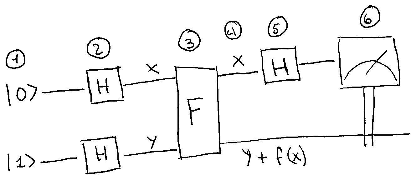
The last gate at the right in the circuit is a measurement. As you see, we are measuring just the x qubit. Maybe your confusion is increasing but I promise everything is going to make sense shortly.
Let’s break down the previous circuit in small steps:
The first step is to put the two qubits input into a 0-1 state.
Apply a Hadamard gate to each qubit. As we saw in a previous chapter, the state of each qubit is now the following:
\(x = \frac{1}{\sqrt{2}}(|0\rangle + |1\rangle) \space and \space y = \frac{1}{\sqrt{2}}(|0\rangle - |1\rangle)\)
So the two-qubit product state after the Hadamard gates is:
Now, we apply the transformation F to this two-qubit state as we defined above. If we disassemble the previous two-qubit state, then apply the function F to each of the individual states, and finally regroup the resulting values, we get the following state:
\(\frac{1}{2}(|0\rangle(|0 + f(0)\rangle - |1 + f(0)\rangle) + |1\rangle(|0 + f(1)\rangle - |1 + f(1)\rangle))\)
In order to get a clearer picture of the effect of F (i.e. the previous formula), let’s do some math magic. Let’s notice that if f(0) = 0 then:
The same way, if f(0) = 1 then:
Remember we are working with modulus-2 arithmetic. In general, for f(0) we have:
If you analyze the possible values for f(1) you can come up with a similar formula. Try it by yourself! Now, if we apply this transformation to the previous result of applying F in the circuit, we get the following:
We now throw the second qubit away and only keep the first one. We only needed the second qubit to make the operations reversible and collect the like-terms. This second qubit is called an ancilla qubit because it is not measured. Keep in mind that a part of the first factors of the previous formula belongs to that second qubit. So we get:
\(\frac{1}{\sqrt{2}}(|0\rangle + (-1)^{(f(0) + f(1))}|1\rangle)\)
This is the value of the first qubit.
Apply another Hadamard gate to the previous qubit to produce:
\(\frac{1}{2}((1 + (-1)^{(f(0) + f(1))})|0\rangle + (1 - (-1)^{f(0) + f(1)})|1\rangle))\)Measure the qubit. If f(x) is constant, then the state in the previous formula reduces to zero, while if f(x) is balanced then the state reduces to one. That happens because if f(0) = f(1) then the previous formula is just reduced to zero state. Otherwise, it is reduced to one state.
Note that this algorithm shows a single measurement of the two qubits input instead of doing two evaluations as the classical algorithm. But the best part is that this algorithm straightforwardly extends to functions that take any number of input qubits. If you think about it, this means that one single measurement can tell you whether a function of any size is constant or balanced. Remember that for the multi-bit input case, we need the function f to be either constant or balanced so the quantum algorithm works. For a classical computer to do the same task, it would need to measure each input, which is exponentially slower.
Looking at the horizon
In this season finale, we finally created our first quantum algorithm. The problem we solved is known as the Deutsch-Jozua problem. It has no known commercial applications yet. But other useful quantum algorithms like Shor’s factoring algorithm rely upon similar concepts.
There is a belief in the community that there are quantum algorithms that can speed up Machine Learning training and efficiently simulate the quantum behavior of molecules.
As of November 2022, IBM has built the most powerful quantum computer that exists. It is the IBM Osprey and has 433 qubits. Companies like Google and IBM are working hard to build powerful quantum computers. They believe in the usefulness of Quantum Computing. For example, factoring a 1024-bit modern encryption key using Shor’s algorithm would require more than 5,000 qubits! This is far from the current state of the art. We know there are problems that quantum computers can solve faster, but the usefulness of Quantum Computing depends on the existence of more powerful quantum computers.
This is the end of our first season of Towards Quantum Computing. I hope you have learned a lot. But, what is still to come? Well, it would be great to have a deeper knowledge of the quantum nature of atoms and particles. We take that nature for granted but we haven’t explored how this nature is manifested in the real world. This will allow us to understand better what is a qubit, which is also a pending issue. Another interesting topic is to explore the different complexity classes of problems and how Quantum Computing influences this classification.
But my greatest debt is to show an actual implementation (i.e. shutting up and showing the code) of a quantum algorithm. There are some SDKs available out there that let us experiment with quantum computing. I would love to include it in this season but it won’t happen as it requires more time from me. However, it is my top priority for the next season.
Now is your turn, what do you think about this first season of the series? Did you like it? What other topics you’d like to read about next season? Do you even want a new season? Please, let me know the answer by replying to this post. I will appreciate it a lot. You can also hit that heart button and share Under the Hype with your friends. Have a nice week, and be prepared for more Computer Science!
See you!